This blog is wroten with the help of Yuanqi Du and Yanbang Wang. See full contents in AI4science blog 101
Before you start
Graph is the fundamental data structure that denotes pairwise
relationships between entities across various domains, e.g., web, gene,
and molecule. Machine learning on graph, typical on Graph Neural
Network, becomes more and more popular in recent years. In this blog, we
will introduce some basic concepts of machine learning on graph. We hope
it may give you inspiration on:
-
what is graph? why do we need graph? How to solve graph-related
problems with machine learning techniques?
-
How to correlate your specific task with the graph and view it as a
graph problem?
-
How to utilize existing techniques to solve your specific task?
Before going deep into the technical details, we first provide some
motivations by introducing some histories on the developement of graph
Neural Network (GNN). The history of GNN is emerged as a response to two
significant challenges. The first challenge came from the data mining
domain, where researchers were exploring ways to extend deep learning
techniques to handle structured network data. Examples of such data
include the World Wide Web, relational databases, and citation networks.
The second challenge arose from the science domain, where researchers
were attempting to apply deep learning techniques to practical science
problems such as single-cell analysis, brain network analysis, and
molecule property prediction. To meet these practical challenges, the
GNN community has grown rapidly, with researchers collaborating across
different fields beyond data mining.
Graph type, Graph task, towards Graph modeling
What are graphs? Why are graphs ubiquitous in science?
What are graphs?
The graph is a data formulation that is widely utilized to describe
pairwise relations between nodes. Mathematically, a graph can be denoted
as \(\mathcal{G}=\left \{\mathcal{V}, \mathcal{E} \right \}\).
\(\mathcal{V}= \left \{v_1, v_2, \cdots, v_N \right \}\) is a set of
\(N=\left | \mathcal{V} \right |\) nodes.
\(\mathcal{E}= \left \{e_1, e_2, \cdots, e_M \right \}\) is a set of
\(M=\left | \mathcal{E} \right |\) which describes the connections between
nodes. \(e=(v_1, v_2)\) indicates there is an edge exists from node \(v_1\)
to node \(v_2\). Moreover, nodes and edges can have corresponding features
\(X_V\in \mathbb{R}^{N\times d}\), \(X_E\in \mathbb{R}^{M\times d}\),
respectively.
Why are graphs ubiquitous in science?
The main advantage of the graph formulation is the universal
representation ability.
Universal represents that graph can be a natural representation for
arbitrary data. In the data mining domain, much data can be naturally
represented as a graph. Examples are shown in
Figure 1
-
Social network [1] can be represented as a
graph. Each node represents one user. Each edge indicates that the
relationship exits between two users, e.g., friendship, domestic
relationship,
-
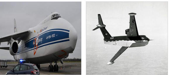
Transport Network [2] can be represented as a
graph. Each node represents one station. Each edge indicates that a
route exists between two stations.
-
Web Network [3] can be represented as a graph.
Each node represents one web page. Each edge indicates that a
hyperlink exists between two pages.

(a) Social Network
|

(b) Transport Network
|

(c) Web Network
|
Figure 1: Examples for graph data in data mining domain
Moreover, the graph can also generalize into different domains. In the
computer vision domain, The image can be viewed as a grid graph. In the
natural language processing domain, the sentence can be viewed as a path
graph. IN AI4Science, the graph can adapt to all scientific problems
easily. More concrete examples are shown in Figure 2
-
Brain network [4] can be represented as a graph.
Nodes represent brain regions, and edges represent connections
between them. Connections can be structural, such as axonal
projections, or functional, such as correlated activity between
brain regions. Brain network graphs can be conducted with different
scales, ranging from individual neurons and synapses to large-scale
brain regions and networks.
-
Gene-gene network [5] can be represented as a
graph. In a gene-gene network, nodes represent genes, and edges
represent interactions between them. These interactions can be based
on different types of experimental evidence, such as co-expression,
co-regulation, or protein-protein interactions. Gene-gene networks
can be conducted with different levels of complexity, from small
subnetworks involved in specific biological pathways to large-scale
networks that span the entire genome.
-
Molecule network [6] can be represented as a graph.
chemical compounds are denoted as graphs with atoms as nodes and
chemical bonds as edges. Molecular networks can be conducted with
different levels of complexity, from simple compounds such as water
and carbon dioxide to complex biomolecules such as proteins and DNA.

(a )Gene-gene Network
|

(b) Brain Network
|

(c) Molecule Network
|
Figure 2: Examples for graph data in AI4Science domain
The simple graph mentioned in
Section [1.1] shows the most basic formulation of the graph
which only takes single node and edge type into consideration. However,
different data may have additional features which cannot be easily
handled on the single graph formulation.
In this subsection, we will briefly describe popular complex graphs
including the heterogeneous graph, bipartite graph, multidimensional
graph, signed graph, hypergraph, and dynamic graph.
Bipartite Graph
The bipartite graph formulation is a special single graph where edges
can only between two node sets \(\mathcal{V}_1\) and \(\mathcal{V}_2\). Two
node sets should have: (1) no overlap between two node sets:
\(\mathcal{V}_1 \cap \mathcal{V}_2 = \emptyset\). (2) contains all nodes:
\(\mathcal{V}_1 \cup \mathcal{V}_2 = \mathcal{V}\). The bipartite graph is
utilized to describe the interactions between different objectives. It
is typically utilized in the e-commerce system to describe the
interaction between users and documents. It can also be utilized on
different science problems.
Signed Graph
The signed graph is introduced to describe the graph with two edge
types: positive edges and negative edges. A signed graph \(\mathcal{G}\)
consists of a set of nodes \(\mathcal{V}=\{v_1, \cdots, v_N \}\) and a set
of edges \(\mathcal{E}=\{e_1, \cdots, e_M \}\). Additionally, there is an
edge-type mapping function \(\phi_e:\mathcal{E}\to\mathcal{T}_e\) that map
each edge to their types, positive or negative.
\(\mathcal{T}_e = \left \{1, -1 \right \}\) indicate the edge type,
positive or negative. It is typically utilized in social networks like
Twitter, where the positive edge indicates following, and the negative
edge indicates block or unfollow. It can also be utilized on different
science problems.
Heterogeneous Graph
The heterogeneous graph introduced more node types on the graph. New
relationship types can also be found as edges can be found between
different node types.
For example, the simple citation network can be represented with the
single graph formulation, where each node represents a paper, each edge
represents one paper cites another one. However, the citation network
can be more complex when considering: (1) authors. authors could have a
co-author relationship. The author could also write papers. (2) Paper
types. Paper can have different types, e.g., Data Mining, Artificial
Intelligence, Computer Vision, and Natural Language Processing.
A Heterogeneous graph \(\mathcal{G}\) consists of a set of nodes
\(\mathcal{V}=\{v_1, \cdots, v_N \}\) and a set of edges
\(\mathcal{E}=\{e_1, \cdots, e_M \}\). Additionally, there are two mapping
functions \(\phi_n:\mathcal{V}\to\mathcal{T}_n\),
\(\phi_e:\mathcal{E}\to\mathcal{T}_e\) that map each node and each edge to
their types, respectively. \(\mathcal{T}_e\) indicate the set of node an
edge type.
Multidimensional Graph
Multidimensional graph is introduced to describe multiple relationships
that simultaneously exist between a pair of nodes. It is different from
the signed graph and the heterogeneous graph that both of them do not
allow multiple edges between a pair of nodes. A multidimensional graph
consists of a set of \(N\) nodes \(\mathcal{V}= \{v_1, \cdots, v_n \}\) and
\(D\) sets of edges \(\{\mathcal{E}_1, \cdots, \mathcal{E}_D \}\). Each edge
set \(\mathcal{E}_d\) describes the \(d\)th type of relation between nodes.
The intersection between different edge sets is allowed. It is typically
utilized in the social network. Users can "like", "Retweet", and
"comment" on the tweet. Each action corresponds to one relationship
between user and tweet. It can also be utilized on different science
problems.
Hypergraph
The hypergraph is introduced when you are required to consider the
relationship beyond a pair of nodes. A hypergraph \(\mathcal{G}\) consists
of a set of \(N\) nodes \(\mathcal{V}= \{v_1, \cdots, v_n \}\) and a set of
hyperedges \(\mathcal{E}\). The incident matrix
\(\mathbf{H} \in \mathbb{R}^{|\mathcal{V}|\times |\mathcal{E}| }\) instead
of using the adjacent matrix \(\mathbf{A}\) is utilized to describe the
graph structure.
\[H_{i j} = \begin{cases}
1 & \text{if vertex } v_{i} \text{ is incident with edge } e_{j} \\
0 & \text{otherwise.}
\end{cases}
\tag{1}\]
It is typically utilized in the academic network.
where nodes are papers and authors. One author can publish more than one
paper which can be viewed as a hyper-edge connecting multiple papers.
Dynamic Graphs
Dynamic graph is introduced when the graph constantly evolves where new
nodes and edges may be added and some existing nodes and edges may
disappear in the graph. A dynamic graph \(\mathcal{G}\) consists of a set
of \(N\) nodes \(\mathcal{V}= \{v_1, \cdots, v_n \}\) and a set of edges
\(\mathcal{E}\) where each node and edge is associated with a timestamp
indicating the time it emerged. We have two mapping functions \(\phi_v\),
and \(\phi_e\) mapping each node and each edge to the timestamps,
respectively. It is typically utilized in the social network, where
nodes are users on Twitter. There are new users every day and they can
follow and unfollow other users from time to time.
Knowledge Graph
Knowledge Graph is an important application on the graph domain. It is
comprised of nodes and edges, where nodes \(\mathcal{V}\) represent
entities (such as people, places, or objects) and edges \(\mathcal{E}\)
represent relationships \(\mathcal{R}\) between these entities. These
relationships can be diverse, including semantic relations (e.g., "is
a" or "part of"), factual associations (e.g., "born in" or "works
at"), or other contextual links. The graph-based structure allows for
efficient querying and traversing of data, as well as the ability to
infer new knowledge by leveraging existing connections.
A Knowledge Graph is a structured representation of information that
aims to model the relationships between entities, facts, and concepts in
a comprehensive and interconnected way. It provides a flexible and
efficient means of organizing, querying, and deriving insights from
large volumes of data, making it a powerful tool for information
retrieval and knowledge discovery. It is widely utilized in the Semantic
web which enables machines to better understand and interact with web
content by organizing information in a machine-readable format.
Remark: In this subsection, we briefly introduce different graph
formulations in this subsection. However, the real-world case could be
more complicated. For example, The Network in E-commerce could be a
Heterogeneous bipartite multidimensional graph. It typically corresponds
to the following scenarios: (1) Heterogeneous: Customer and purchaser
could be different user types. Different items also have different
types. (2) bipartite: Users could only have interactions with the items.
(3) multidimensional: Users could have different interactions on the
items, e.g., "buy" "add to shopping cart", and so on.
The graph formulations described in this subsection are more like
prototypes. You can design the typical graph formulation for your data.
It could be easy to learn from the recent progress on the corresponding
graph type to your data.
What are typical tasks on graph?
In this subsection, we provide a brief introduction on the graph-related
tasks to show how we can utilize the graph on different scenarios. We
typically introduce node classification, graph classification, graph
generation, link prediction tasks. Most downstream tasks can be viewed
as an instance for the above tasks
Node Classification
Node classification aims to identify which class the graph node should
belong by utilizing the ego feature, adjacent matrix, and features from
other nodes. The node classification task has numerous real-world
applications. Examples are as follows: (1) social network analysis: In
social networks, nodes and edges represent each individual and social
relationships. Node classification can be utilized to predict various
attributes, such as interests, affiliation, profession and so on. (2)
Bioinformatics: In biological networks, nodes represent genes, proteins,
or other biological entities, and the connections between nodes
represent interactions such as regulatory or metabolic relationships.
Node classification can be utilized to predict various node properties,
such as the function, localization, or disease association. (3)
Cybersecurity: In network security, nodes represent computers, servers,
or other network devices, and the connections between nodes represent
communication or access relationships. Node classification can be
utilized to detect various types of network attacks or anomalies, such
as malware, spam, or intrusion attempts.
Graph Classification
Graph classification aims to identify which class the graph should
belong with exploiting both rich information from the graph structure
and the node feature. Image classification can be viewed as a special
case for the graph classification task. Each pixel can be viewed as a
node, where RGB is the corresponding node feature. The graph structure
on image is a grid which connects the adjacent pixels. Graph
classification has been broadly utilized in many real-world
applications. Examples are shown as follows. (1) bioinformatics: The
graph classification can be utilized to identify biological networks
into different categories. For example, we could classify a set of
protein-protein interaction networks based on their function or disease
association. It can help identify potential drug targets, protein
complexes, or pathways, and inform drug discovery. (2) chemistry: The
graph classification can be utilized to identify chemical compounds into
different categories. For example, we could classify a set of compounds
based on their toxicity or therapeutic potential. (3) Social Network
Analysis: Graph classification can be utilized to identify the
discussion topic of a tweet in Twitter.
Link Prediction
Link prediction can be viewed as a binary classification task predicting
whether there is a link exists between two nodes on the graph. It could
complete the graph and find the under-discovered relationship between
nodes. Link prediction has been broadly utilized in many domains.
Examples are shown as follows: (1) Friend recommendation in the social
network. Twitter could recommend you some friends you may know or
interested in. (2) Movie recommendation. Netflix will recommend you the
film you may be interest in. (3) bioinformatics: In biological networks,
link prediction can be utilized to predict the likelihood of physical
interactions between pairs of proteins based on their sequence
similarity, domain composition, or other features. It can help identify
potential drug targets, protein complexes, or pathways, and inform drug
discovery.
Graph Generation
In contrast to the aforementioned tasks, graph generation aims to solve
the generative problem: given a dataset of graphs, learn to sample new
graphs from the learned data distribution. As graph could represent many
highly-structured data, graph generation has the promises for design
tasks in a variety of domains such as molecular graph generation (drug &
materials discovery), circuit network design, in-door layout design,
etc.
How to Model Graph Structured Data?
In this section, we aim to introduce (1) the Graph Neural Networks which
have become popular for learning graph representations by jointly
leveraging attribute and graph structure information. (2) understanding
perspectives on GNN which connect GNN design to other domains, e.g.,
graph signal process, Weisfeiler-Lehman Isomorphism Test, and so on (3)
traditional graph machine learning methods and structure-agnostic
methods which may perform even better than GNN
Graph Neural Network
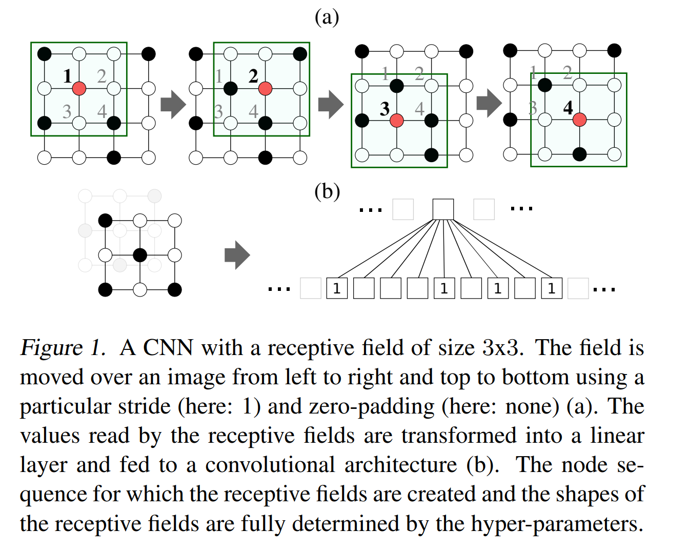
The design of Graph Neural Network is inspired from the Convolution
Neural Network which is one of the most widely-used Neural Networks in
the computer vision domain. It takes effort to utilize the neighborhood
pixel to learn a good representation. Concretely speaking, convolutional
Neural Networks extract different feature patterns by aggregating the
neighboring pixels in a fixed-size receptive field, for example, a
receptive field with \(3\times 3\) neighborhood pixels. To extend the
superiority of CNN to the graph, researchers develop the Graph Neural
Network. There are two essential problems in developing the Graph Neural
network.
Those two questions lead to two crucial perspectives on designing Graph
Neural Networks, spectral and spatial perspectives, respectively. Before
going into the details in those details, we first provide a definition
of the general Graph Neural Network Framework.
A General Framework for Graph Neural Network
We introduce the general frameworks of GNNs for the most basic
node-level task. We first recap some notations on the graph. We denote a
graph as
\(\mathcal{G}= \left \{ \mathcal{V}, \mathcal{E} \right \}\) (i.e.
molecule). The adjacent matrix and the associated features are denoted
as \(\mathbf{A}\in \mathbb{R}^{N \times N}\) (i.e. bond type) and
\(\mathbf{F}\in \mathbb{R}^{N \times d}\) (i.e. atom type), respectively.
\(N\) and \(d\) are the numbers of nodes and feature dimensions,
respectively.
A general framework for Graph Neural Networks can be regarded as a
composition of \(L\) graph filter layers, and \(L-1\) nonlinear activation
layers. \(h_i\) and \(\alpha_i\) are utilized to denote the \(i\)-th graph
filter layer, and activation layer, respectively.
\(\mathbf{F}_i \in \mathbb{R}^{N\times d_i}\) denotes the output of the
\(i\)-th graph filter layer \(h_i\). \(\mathbf{F}_0\) is initialized to be the
raw node features \(\mathbf{F}\).
Spatial Graph filter: How to define the receptive field?
For the image with a regular grid structure, the receptive fields are
defined as the neighborhood pixel around the central pixel. An example
is illustrated in Fig. . So how to define the receptive field on the
graph with no unified regular structure? The answer is the neighborhood
nodes along the edge. One hop neighborhood of node \(v_i\) can be defined
as
\(\mathcal{N}_{v_i} = \left \{ v_j s.t., (v_i, v_j) \in \mathcal{E}\right \}\).
To adaptively extract the neighborhood information, a large variety of
spatial-based graph filters are proposed. We introduce two typical
spatial Graph-filter layers, GraphSAGE and GAT, in this section.
GraphSAGE [7]: The GraphSAGE model proposed in
() introduced a spatial-based filter that aggregation information from
neighboring nodes. The hidden feature for node \(v_i\) is generated with
the following steps.
-
Sample neighborhood nodes from the neighborhood set.
\(\mathcal{N}_S(v_i)=\text{SAMPLE}(\mathcal{N}(v_i), S)\)
where
\(\text{SAMPLE}()\) is a function that takes the neighborhood set as
input, and random sample \(S\) instances as the output.
-
Extract the information from neighborhood nodes.
\(f_i' = \text{AGGREGATE}( \left \{ \mathbf{F}_j, \forall v_j \in \mathcal{N}_S(v_i) \right \} )\)
where \(\text{AGGREGATE}: \mathbb{R}^{M\times d} \to \mathbb{R}^{d}\)
is a function to combine the information from the neighboring nodes.
-
combine the neighborhood information with the ego information
\(\mathbf{F}_i=\sigma \left ( [\mathbf{F}_i, \mathbf{f}'_i] \mathbf{\Theta} \right )\)
where \([\cdot, \cdot]\) is the concatenation operation, \(\Theta\) is
the learnable parameters.
The aggregation can be a set function with different aggregators
including mean, maximum aggregators, which takes the element-wise mean,
and maximum operator. sum aggregator is later introduced by () with
stronger expressive ability.
GAT [8]: The Graph Attention Network (GAT) is
inspired by the self-attention mechanism. GAT adaptively aggregates the
neighborhood information based on the attention score. The hidden
feature for node \(v_i\) is generated with the following steps.
-
generates the attention score with the neighborhood node.
\(a(\mathbf{F}_i\mathbf{\Theta}, \mathbf{F}_j\mathbf{\Theta})=\text{LeakyReLU} (\mathbf{a}^T \left [ \mathbf{F}_i\mathbf{\Theta}, \mathbf{F}_j\mathbf{\Theta} \right ]) \text{s.t.},v_j \in \mathcal{N}(v_i) \cup \left \{ v_i \right \}\)
where \(a\) is a
-
normalizes the attention score via softmax.
\(\alpha_{ij} = \frac{\exp{e_{ij}}}{\sum_{v_k \in \mathcal{N}(v_i) \cup \left \{ v_i \right \}} \exp{e_{ik}}}\)
-
aggregation the weighted information from neighborhoods.
\(\mathbf{F}'_i = \sum_{v_j \in \mathcal{N}(v_i) \cup \left \{ v_i \right \}} \alpha_{ij}\mathbf{F}_i\mathbf{\Theta}\)
-
multi-head attention implementation.
\(\mathbf{F}'_i = ||_{m=1}^M \sum_{v_j \in \mathcal{N}(v_i) \cup \left \{ v_i \right \}} \alpha_{ij}^m \mathbf{F}_j \mathbf{\Theta}^m\)
Where \(||\) is the concatenation operator, \(M\) is the number of
heads.
Notice that, the key difference between the GAT and self-attention
mechanism is that, self-attention is conducted on all the nodes, where
the GAT is conducted on the neighborhood nodes. More discussion can be
found in the next section.
Spectral Graph filter: What feature patterns are useful on the graph?
Spectral-based Graph Filters majorly utilize the spectral graph theory
to develop the filter operation in the spectral domain. We will only
provide some motivations for Spectral-based Graph Filters without
mathematical details.
The motivation behind spectral graph filters is that neighboring nodes
in a graph should have similar representations. In the context of
spectral graph theory and filters, neighborhood similarity corresponds
to the low-frequency components which changes in the graph structure
that occur slowly or gradually. Contrastively, high-frequency components
correspond to rapid or abrupt changes. By focusing on the low-frequency
components, spectral graph filters can capture the underlying smooth
variations in the graph topology, which can be useful for various tasks
e.g., node classification, link prediction, and graph clustering.
In other words, spectral graph filters aim to identify feature patterns
that are smooth and do not vary significantly across different nodes. It
corresponds to the low-frequency components of the graph structure based
on spectral graph theory.
GCN [9]: We only provide a brief introduction on the
formulation of the Graph Convolutional Network (GCN). A more
comprehensive study can be found in Section 5.3.1 of Deep Learning on
Graphs [10].
The aggregation function of GCN is defined as:
\(\mathbf{F}'= \sigma( \tilde{\mathbf{D}}^{-\frac{1}{2}} \tilde{\mathbf{A}} \tilde{\mathbf{D}}^{-\frac{1}{2}}\mathbf{F}\mathbf{\Theta}) \tag{2}\)
where \(\sigma\) is the activation function,
\(\tilde{\mathbf{D}}^{-\frac{1}{2}} \tilde{\mathbf{A}} \tilde{\mathbf{D}}^{-\frac{1}{2}}\)
is the symmetric normalized adjacent matrix.
The aggregation function for each edge can be defined as:
\(\mathbf{F}'_i = \sum_{v_j \in \mathcal{N}(v_i) \cup \left \{ v_i \right \}}
\frac{1}{\sqrt{\tilde{d}_i\tilde{d}_j}}
\mathbf{F}_j\mathbf{\Theta}\tag{3}\)
where \(\tilde{d}_i\) is the degree of
node \(i\).
Message Passing Neural Network
The above discussion focused on GNN design for the simple graph with a
single node and edge type. Message Passing Neural Network (MPNN) is then
proposed as a more general framework that could cover the entire design
space for GNNs. Concretely speaking, MPNNs are a family of neural
networks that operate on graphs by (1) generating messages between nodes
based on their local neighborhoods. (2) aggregating messages from
neighboring nodes iteratively to MPNNs can learn powerful graph
representations for various downstream tasks.
The above discussion focuses on the GNN design on the simple graph with
single node and edge type. Message Passing Neural Network is a re A more
general Graph Neural Network. Message passing Neural Network is a more
general framework which could cover the whole design space for GNN.
The Message Passing filter can be defined as:
\(h_{i}^{\ell+1}=\phi\left(h_{i}^{\ell}, \oplus_{j \in \mathcal{N}_{i}}\left(\psi\left(h_{i}^{\ell}, h_{j}^{\ell}, e_{i j}\right)\right)\right)\tag{4}\)
where \(\phi\), \(\psi\) are Multi-Layer Perceptrons (MLPs), and \(\oplus\) is
a permutation-invariant local neighborhood aggregation function such as
summation, maximization, or averaging.
Focusing on one particular node \(i\), the MPNN layer can be decomposed
into three steps as:
-
Message: For each pair of linked nodes \(i\), \(j\), the network
first computes a message
\(m_{i j}=\psi\left(h_{i}^{\ell}, h_{j}^{\ell}, e_{i j}\right)\) The
MLP \(\psi: \mathbb{R}^{2d+d_e}\to \mathbb{R}^{d}\) takes as input the
concatenation of the feature vectors from the source node, target
node, and edge feature.
-
Aggregate: At each source node \(i\), the incoming messages from
all its neighbors (target node) are then aggregated as
\(m_{i}=\oplus_{j \in \mathcal{N}_{i}}\left(m_{i j}\right)\)
-
Update: Finally, the network updates the node feature vector
\(h_{i}^{\ell+1}=\phi\left(h_{i}^{\ell}, m_{i}\right)\) by
concatenating the aggregated message \(m_i\) and the previous node
feature vector \(h_i^{\mathcal{l}}\), and passing them through an MLP
\(\phi: \mathbb{R}^{2 d} \rightarrow \mathbb{R}^{d}\).
Permutation Equivaraince/Invariance
A function \(f\) is said to be equivariant if for any transformation
\(\tau\) of the input space \(X\), and any input \(x\in X\), we have:
\(f(\tau(x)) = \tau(f(x))\). In other words, applying the transformation
\(\tau\) to the input has the same effect as applying it to the output. A
function \(f\) is said to be invariant if for any transformation \(\tau\) of
the input space \(X\), and any input \(x\in X\), we have:
\(f(\tau(x)) = f(x)\). In other words, applying the transformation \(\tau\)
to the input does not change the output.
In the context of GNNs, we want to achieve permutation-equivariance or
permutation-invariance, which means that the function should be
equivariant or invariant to permutations of the input graph. We can
express this mathematically by defining a permutation \(\sigma\) of the
nodes of the input graph \(G=(V,E)\), and requiring that the output of the
GNN is the same regardless of the permutation: \(f(G) = f(\sigma(G))\),
where \(\sigma(G)\) is the graph obtained by applying the permutation
\(\sigma\) to the nodes of \(G\).
Understanding perspectives on GNN

Figure 3: An overview of the connection between WL-test and Graph Neural Network. Middle panel: rooted subtree structures (at the blue node) that the WL test uses to distinguish different graphs. Right panel: if a GNN’s aggregation function captures the full multiset of node neighbors, the GNN can capture the rooted subtrees in a recursive manner and be as powerful as the WL test[11]
GNN Expressiveness and Weisfeiler-Lehman Isomorphism Test.
The expressiveness of Graph Neural Network is highly related with the
graph isomorphism test. An expressive GNN should map the isomorphic
graphs into the same representation and distinguish non-isomorphic
graphs with different representations.
The Weisfeiler-Lehman (WL) test is a popular graph isomorphism test used
to determine whether two graphs are isomorphic, meaning two graphs have
the same underlying structure but may differ in the node labeling. The
intuition for WL-test is that if two graphs are isomorphic, then their
structures should be similar across all hops of neighborhoods, from
one-hop neighborhoods to the global structure of the entire graph. The
algorithm iterates on the following two steps: (1) aggregation: collect
a set of neighbor node labels (2) labeling: assigned a new label based
on the label set of neighbor nodes. The WL-test will repeat this
labeling and aggregation process until convergence (node label does not
change). We can then identify whether two graphs are isomorphic if they
have the same sequence of refined graphs or not. The WL-test is widely
utilized in different domains since it is efficient with the time
complexity \(O(n \log (n))\), where \(n\) is the number of the nodes. More
recently, the WL-test is widely utilized for analyzing the
expressiveness of GNN.
Graph Neural Networks and Transformer architectures are typically two
popular model architectures to leverage the context information.
Connections can be found between those two architectures.
\(\begin{array}{c}
h_{i}^{\ell+1}=\operatorname{Attention}\left(Q^{\ell} h_{i}^{\ell}, K^{\ell} h_{j}^{\ell}, V^{\ell} h_{j}^{\ell}\right), \\
i . e ., h_{i}^{\ell+1}=\sum_{j \in \mathcal{S}} w_{i j}\left(V^{\ell} h_{j}^{\ell}\right),
\end{array}\)
where \(w_{i j}=\operatorname{softmax}_{j}\left(Q^{\ell} h_{i}^{\ell} \cdot K^{\ell} h_{j}^{\ell}\right)\). \(j\in \mathcal{S}\) denotes the set of words in the sentence
\(\mathcal{S}\) and \(Q^{\mathcal{l}}, K^{\mathcal{l}}, V^{\mathcal{l}}\)
are learnable linear weights. Three matrices denote the Query, Key, and
Value for the attention respectively. One update on each word embedding
can be viewed as a weighted aggregation of all word embeddings in the
sentence. An illustration of self-attention block in Transformer is
shown in
Fig. 4(b)
One Graph Neural Network block can be defined as follows:
\(h_{i}^{\ell+1}=\sigma\left(U^{\ell} h_{i}^{\ell}+\sum_{j \in \mathcal{N}(i)}\left(V^{\ell} h_{j}^{\ell}\right)\right),\tag{5}\)
where \(U^{\mathcal{l}}, V^{\mathcal{l}}\) are learnable transformation
matrices of the GNN layer and \(\sigma\) is the non-linearity activation
function. One update for the hidden representation \(h_i\) of node \(i\)at
layer \(\mathcal{l}\) be viewed as a weighted aggregation of neighborhood
nodes representation \(j\in \mathcal{N}(i)\).
An illustration of GNN block is shown in
Fig. 4(a)

(a) GNN block
|

(b) Transformer block
|
Figure 4. GNN vs Transformer
The key difference between Graph Neural Network and transformer is that
Graph Neural Network only aggregates on the neighborhood nodes, while
Transformer will aggregate on all the words in the sentence. In another
word, Transformer can be viewed as a GNN aggregated on a fully-connected
word graph. In other words, both Graph Neural Network and Transformer
aim to learn good representation by incorporating context information.
Transformer recognizes all the words in one sentence are useful while
GNN only recognizes that the neighborhood nodes are useful.
GNN and Graph Signal Denoising Processes.
Graph signal denoising [12] offers a new perspective to
create a uniform understanding on representative aggregation operations.
The graph signal denoising is to recover a clean signal from the
original noisy signal. It can be defined as solving the following
optimization problem:
\(arg \min_F \mathcal{L}=||F-S||_F^2 + c \cdot \text{tr}(F^TLF) \tag{6}\)
where \(S\in \mathbb{R}^{N\times d}\) is a noisy signal (input feature) on graph
\(\mathcal{G}\). \(F\in \mathbb{R}^{N\times d}\) is the clean signal assumed
to be smooth over \(\mathcal{G}\).
The first term guides \(F\) to be close to \(S\), while the second term
\(tr(F^TLF)\) is the Laplacian regularization which guides \(F\)’s
smoothness over \(\mathcal{G}\), with \(c > 0\)’s mediation. Assuming that
we adopt the unnormalized version of Laplacian matrix with \(L = D - A\)
(the adjacency matrix \(A\) is assumed to be binary), the second term can
be written in an edge-centric way as:
\(c \sum_{(i,j)\in \mathcal{E}} ||F_i-F_j||_2^2\tag{7}\)
which leads to the
connected nodes sharing similar features.
We show the connection between the graph signal process and GCN as an
example here. The gradient with respect to \(F\) at \(S\) is
\(\frac{\partial \mathcal{L}}{\partial F} \|_{F = S} = 2cLS\)
Hence, one-step gradient descent for the graph signal denoising
problem equation [8] can be described as:
\begin{aligned}
F \leftarrow S - b\left. \frac{\partial \mathcal{L}}{\partial F} \right|_{F = X} &= S - 2bcLS \nonumber
&= (1-2bc )S+ 2bc\tilde{A}S.
\end{aligned}
When stepsize \(b=\frac{1}{2c}\) and \({ S}={ X}'\),
we have \(F \leftarrow \tilde{A}X'\), which is the same as
the aggregation operation of GCN. It provides a new perspective to
understand existing GNNs as a tradeoff between the original feature
preservation and neighborhood smoothness. Moreover, it inspires us to
derive new Graph Neural Networks from different graph signal processing
methods.
GNN and Gradient Flow.
A new physical-inspired perspective is to understand Graph Neural
Network as a discrete dynamical system of particle [13]. Each
node on the graph corresponds to one particle while the edge represents
pair-wise interactions between nodes. The positive and negative
interactions between nodes could be interpreted as attraction and
repulsion between particles, respectively.
To view Graph Neural Network as a discrete dynamical system, one can
correspond the input forward layer by layer as the input evolution by a
system of differential equations. Each discrete time step in the dynamic
system corresponds to one layer forward process.
Gradient flow is a special type of evolution equation of the form
\(f(X(t))=- \nabla \mathcal{E}(X(t))\tag{9}\)
where \(\mathcal{E}\) is an energy
functional, which could be different for different GNNs. The gradient
flow makes \(\mathcal{E}\) monotonically decrease during the evolution.
Simple GNN can be viewed as the gradient flow of the Dirichlet energy
\(\mathcal{E}^{\text{DIR}} =\frac{1}{2} \text{trace}(X^TLX)\tag{10}\)
The
Dirichlet energy measures the smoothness of the features on the graph.
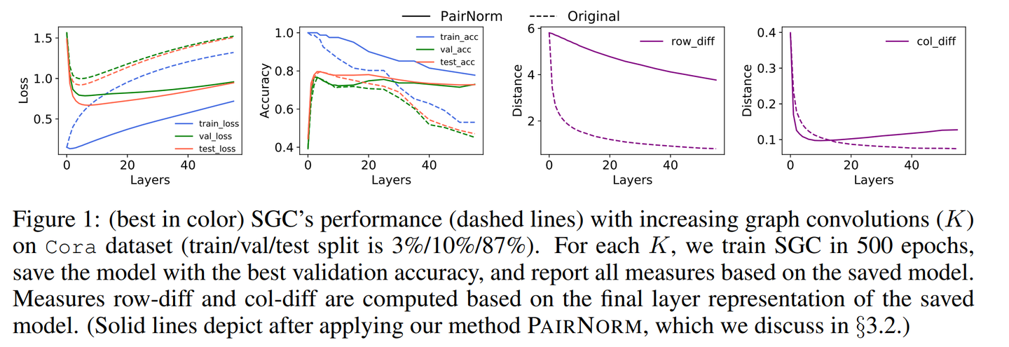
In the limit \(t\to \infty\), all node features is extremely smooth that
all the nodes become the same. It indicates that the system loses the
information contained in the input features. This phenomenon is called
‘oversmoothing’ in the GNN literature.
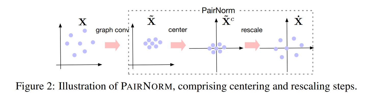
To design better Graph Neural Network to overcome drawback like
oversmooth, we can parametrise an energy and deriving a GNN as its
discretised gradient flow. It offers better interpretability and leads
to more effective architectures.
GNN and Dynamic Programming
Dynamic programming on graphs is a technique that involves solving
problems by breaking them down into smaller subproblems and finding
optimal solutions to those subproblems. This approach can be used to
solve a wide range of problems on graphs, including shortest path
problems, maximum flow problems, and minimum spanning tree problems.
Such an approach shares the similar idea with the aggregation operation
on GNN which recursively combines information from neighboring nodes to
update the representation of a given node. Both GNN aggregation and
dynamic programming on graphs involve combining information from
neighboring nodes to update the representation of a given node. In
dynamic programming, the combination of information is typically done by
recursively solving subproblems and building up a solution to a larger
problem. Similarly, in GNN aggregation, neighboring node information is
combined through various aggregation functions (e.g. mean, max, sum),
and the updated node representation is then passed to subsequent layers
in the network. In both cases, the goal is to efficiently compute a
global solution by leveraging local information from neighboring nodes.
However, vanilla GNNs cannot solve most dynamic programming problems,
e.g., shortest path algorithm, and generalized Bellman-Ford algorithm,
without capturing the underlying logic and structure of the
corresponding problem. To empower GNN with the reasoning ability in
dynamic programming, multiple operators are then proposed to generalize
the operation in dynamic programming to the Neural Network, e.g., the
sum generalizes to a commutative summation operator \(\oplus\), the
product \(\otimes\) generalizes to a Hadamard product operator. GNNs can
then be extended with different dynamic programming algorithms with
improving generalization ability. A simple example of the Graph Neural
Network extending to the Bellman-Ford algorithm can be found in Figure. 4
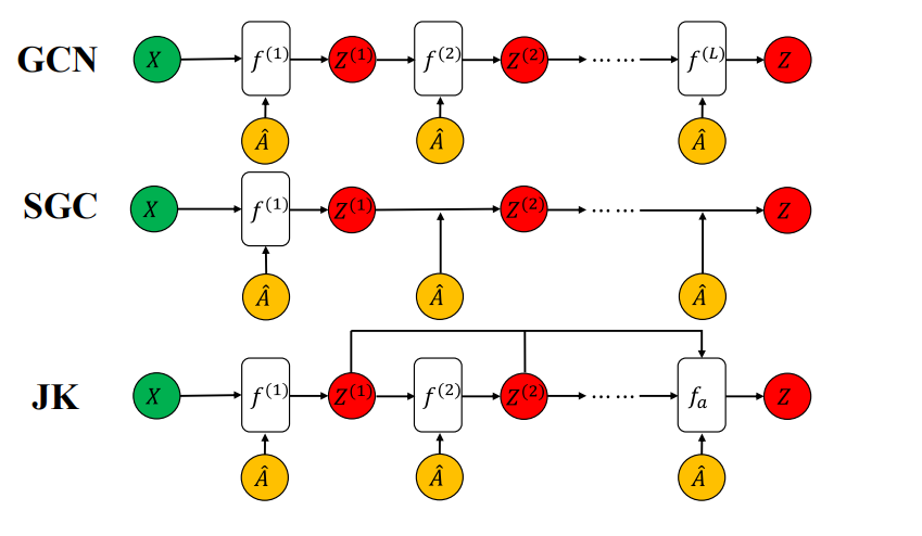
![The framework [14] suggests that better algorithmic alignment
improves generalization. The computation structure of the GNN (left)
aligns well with the Bellman-Ford algorithm (right). GNN can simulate
Bellman-Ford by merely learning a simple reasoning step.](/img/Graph_Machine_Learning/GNN_DP.png)
Figure 5: The framework [14] suggests that better algorithmic alignment
improves generalization. The computation structure of the GNN (left)
aligns well with the Bellman-Ford algorithm (right). GNN can simulate
Bellman-Ford by merely learning a simple reasoning step.
Methods before Graph Neural Network
Graph Neural Network is well-recognized as a powerful method for machine
learning on graph. However, GNN is still not the dominant method in the
graph domain. Traditional machine learning methods on graph and
non-graph methods still reveal advantages over the Graph Neural Network.
They still hold an important position on graph research and inspire the
design of the new Graph Neural Network. In this section, we will first
introduce some important machine learning methods beyond graph including
Graph Kernel methods for graph classification, label propagation for
node classification, and heuristic methods for link prediction.
Label Propagation for node classification
Label Propagation is a simple but effective method for node
classification in graphs. It is a semi-supervised learning technique
that leverages the idea that nodes that are connected in a graph are
likely to share the same label or class. For example, it could be
utilized to a network of people with two labels "interested in
cricket" and "not interested in cricket". We only know the interests
of a few people and we aim to predict the interests of the remaining
unlabeled nodes.
The procedure of label propagation can be found as follows. \(A\) be
the \(n \times n\) adjacency matrix of the graph, where \(A_{ij}\) is 1 if
there is an edge between nodes \(i\) and \(j\), and 0 otherwise. Let \(Y\) be
the \(n \times c\) matrix of node labels, where \(Y_{ij}\) is 1 if node \(i\)
belongs to class \(j\), and 0 otherwise. Let \(F\) be the \(n \times c\)
matrix of label distributions, where \(F_{ij}^{(t)}\) is the probability
of node \(i\) belonging to class \(j\) at iteration \(t\).
At each iteration \(t\), the label distribution \(F^{(t)}\) is updated based
on the label distributions of the neighboring nodes as follows:
\(F^{(t)}=AF^{(t-1)}D^{-1}\tag{11}\)
where \(D\) is the diagonal degree matrix of
the graph, where \(D_{ii} = \sum_j A_{ij}\).
After a certain number of iterations or when the label distributions
converge, the labels of the nodes are assigned according to the label
distribution with the highest probability:
\[Y_i = arg\max_j F^{(t)}_{ij}\tag{12}\]
This process is repeated until the labels converge to a stable state or
until a stopping criterion is met.
\(\hat{\mathbf{Y}}=(\mathbf{D}^{-1}\mathbf{A})^t\mathbf{Y}\tag{13}\)
where
\(\mathbf{D}\) and \(\mathbf{A}\) is the degree matrix and adjacent matrix,
respectively. \(t\) is the number of propagation.
\(\mathbf{Y}=\begin{bmatrix}
\mathbf{Y}_l \\
\mathbf{0}
\end{bmatrix}\) is the vector of labels on nodes.
\(\mathbf{D}^{-1}\mathbf{A}\) is the transition matrix.
Graph kernel methods for graph classification
Graph Kernel method is to measure the similarity between two graphs with
a kernel function which corresponds to an inner product in reproducing
kernel Hilbert space (RKHS). Kernel methods are widely utilized in the
Support Vector Machine. It allows us to model higher-order features in
the original feature space without computing the coordinates of the data
in a higher dimensional space. Graph kernel methods confront additional
challenges than the general kernel methods on how to encode the
similarity on the graph structure. The design of graph kernel methods
focuses on finding suitable graph patterns to measure similarity. We
will briefly introduce the subgraph pattern and path pattern on graph
kernels.
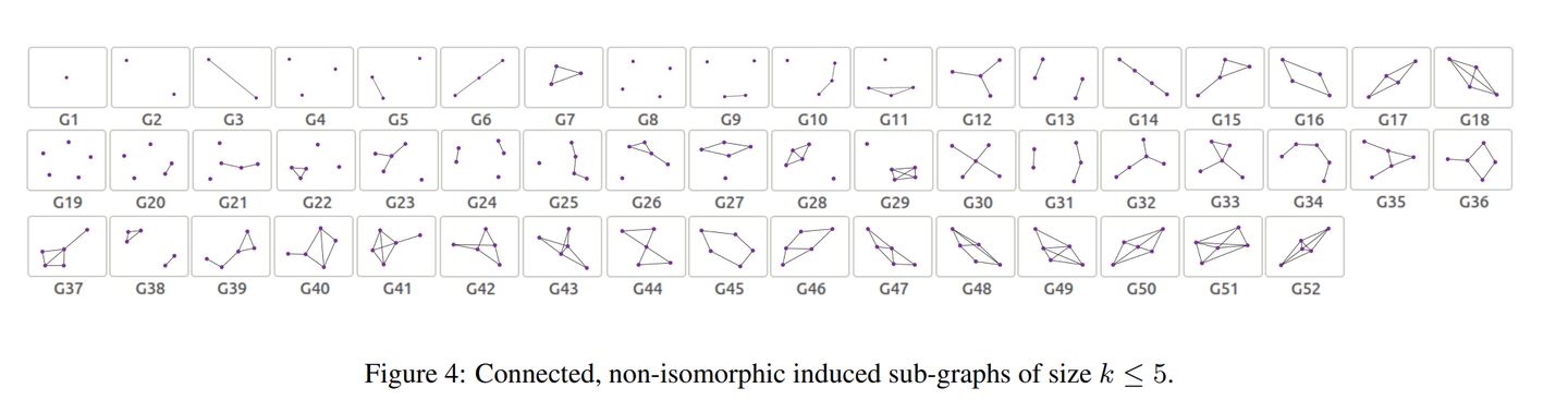
Graph kernels based on subgraphs aims to find the same subgraph
between graphs. Two graphs with more same subgraphs are more similar.
Subgraph set can be defined by the graphlet, which is an induced and
non-isomorphic sub-graph of node size-\(k\). An illustration can be found
in Fig.3 A pattern count vector \(\mathbf{f}\) will be
calculated where \(i^{\text{th}}\) component denotes the frequency of
subgraph pattern \(i\) occurs.
The graph kernel can then be defined as:
\(\mathcal{K}_{\text{GK}}(\mathcal{G}, \mathcal{G}')= \left \langle \mathbf{f}^{\mathcal{G}} \mathbf{f}^{\mathcal{G}'} \right \rangle\)
where \(\mathcal{G}\) and \(\mathcal{G}'\) are two graph,
\(\left \langle \cdot, \cdot \right \rangle\) denotes the Euclidean dot
product.
![Connected, non-isomorphic induced sub-graph of node size $$k \le 5$$.
[15]](/img/Graph_Machine_Learning/graphlet.png)
Figure 6: Connected, non-isomorphic induced sub-graph of node size $$k \le 5$$
Graph kernels based on path decomposes a graph into paths. It takes
the co-occurrence of random-walk on two graphs to calculate the
similarity. Different from the subgraph-based methods focusing on the
graph structure, random-walk based method takes the node label in the
graph into consideration. It counts all shortest paths in graph
\(\mathcal{G}\) denoting as triplets \(p_i=(l_s^i, l_e^i, n_k )\). \(n_k\)is
the length of the path. \(l_s^i\) and \(l_e^i\) are the labels of the
starting and ending vertices, respectively.
Similarly, the graph kernel can be defined as:
\(\mathcal{K}_{\text{GK}}(\mathcal{G}, \mathcal{G}')= \left \langle \mathbf{f}^{\mathcal{G}} \mathbf{f}^{\mathcal{G}'} \right \rangle\tag{15}\)
where the \(i^{\text{th}}\) component of \(\mathbf{f}\) denotes the
frequency of triplet occurring.
Heuristic methods for link prediction
Heuristic methods, i.e., Common Neighbor, utilize the graph structure to
estimate the likelihood of the existence of links. We will briefly
introduce some basic heuristic methods including common neighbors,
Jaccard score, preferential attachment, and Katz index. \(\Gamma(x)\)
denote the neighbor node set of \(x\). \(x\) and \(y\) denote two different
nodes.
Common Neighbors (CN): The Common Neighbors algorithm considers two
nodes with more overlapping neighbor nodes are more likely to be
connected. Common neighbors algorithm calculates the intersection
between neighbor nodes of node \(x\) and node \(y\).
\(f_{\text{CN}}(x,y)=| \Gamma(x) \cap \Gamma(y) |\tag{16}\)
Jaccard score: Jaccard score can be viewed as a normalized Common
Neighbors algorithm, where the normalized factor is union of node sets.
\(f_{\text{Jaccard}}(x,y)=\frac{| \Gamma(x) \cap \Gamma(y) |}{| \Gamma(x) \cup \Gamma(y) |}\tag{17}\)
Preferential attachment (PA): Preferential attachment algorithms
consider that nodes with higher degrees are more likely to be connected.
Preferential attachment calculates the product of node degrees.
\(f_{\text{PA}}(x,y)=| \Gamma(x) | \times | \Gamma(y) |\tag{18}\)
Katz index Katz index algorithm takes high-order nodes into
consideration compared with the above algorithms based on one hop
neighborhood. Katz index considers that nodes with more short paths are
more likely to be connected. It calculates the weighted sum of all the
walks between \(x\) and \(y\) as follows:
\(f_{\text{Katz}}(x,y)= \sum_{l=1}^{\infty}\beta^l |\text{walks}^{\left \langle l \right \rangle }(x,y)|\tag{19}\)
\(\beta\) is a decaying factor between 0 and 1, which gives a smaller
weight to distant path.
\(|\text{walks}^{\left \langle l \right \rangle }\) counts the length
between \(x\) and \(y\).
Applying Graph Machine Learning in Scientific Discovery
In this section, we will first introduce some general tips for applying
graph machine learning in scientific discovery followed by two success
examples in molecular science and social science.
Tips for Applying Graph Machine Learning
efficiency issues on graph
-
If your task focuses on a single large graph, it may meet the
out-of-memory issue. We suggest you (1) utilize sampling
strategies (2) less propagation layer without involving too many
neighbors.
-
If your task focuses on multiple small graphs, time efficiency may
be an issue. (Seems that GNN can be very slow on mini-batch task)
effective issues on graph
-
feature matters: if your graph node does not have the feature, you
can conduct the feature manually. Some suggested features are
degree, Laplacian Eigenvector, DeepWalk embedding.
-
feature normalization may heavily influence the performance of GNN
models.
-
add self-loop may provide additional gain to your model
-
The performance on single data split may not be reliable. Try
different data splits for reliable performance.
when graph may not work
-
If your data does not naturally have the graph structure, it may not
be necessary to conduct graph structure manually to apply GNN
methods on.
-
GNN is a permutation equivalence Neurel Network. It may not work
well on tasks requiring other geometric properties and also nodes
related to other information.
Algorithm 1:
Input: molecule, radius R, fingerprint length S
Initialize:
    fingerprint vector f ← 0_S
    r_a ← g(a)
    r_1 ... r_N = neighbors(a)
    v ← [r_a, r_1, ..., r_N]
    r_a ← hash(v)
    i ← mod(r_a, S)
    f_i ← 1
Return: binary vector f
Algorithm 2:
Input: molecule, radius R, hidden weights H_1^1 ... H_R^5, output weights W_1 ... W_R
Initialize:
    fingerprint vector f ← 0_S
    r_a ← g(a)
    r_1 ... r_N = neighbors(a)
    v ← r_a + Σ_{i=1}^{N} r_i
    r_a ← σ(vH_L^N)
    i ← softmax(r_a W_L)
    f ← f + i
Return: real-valued vector f
Success in Modeling Molecular Structures (Chemistry/Biology)
Molecules are one of the most common applications for graph neural
networks, especially message passing neural networks. Molecules are
naturally graph objects and GNNs provide a compact way to learn
representations on molecular graphs. This line of work has been opened
up by a seminal work NEF [16] where they built a
neat connection between the process of constructing the most commonly
used structure representation (molecular fingerprints) and graph
convolutions. As shown in
Algorithm [2]. It is worth noting that the commonly used
string encoding for molecules (SMILES — Simplified Molecular Input
Line Entry System) could be considered as a parsing tree (implicit graph
representation) defined by the grammar.

Figure 8: Representing crystal structures with GNNs (handling periodicity). (Figure taken from [17])
![Designing protein sequences via a graph-to-sequence model. (Figure taken from [17])](/img/Graph_Machine_Learning/proteinmpnn.png)
Figure 9: Designing protein sequences via a graph-to-sequence model. (Figure taken from [18])
There are mainly two branches of problems that have been discovered
extensively with graph representation and graph neural networks: (1)
predictive task, and (2) generative task. Predictive task refers to
answering a specific question about certain molecules, such as the
toxicity, energy, etc. of any given molecules. This is particularly
beneficial for tasks like virtual screening which otherwise requires
experiments to obtain the property of molecules. On the other hand,
generative task aims to design and discover new molecules with certain
interesting properties which is also called molecular inverse design.
For predictive task, graph representation provides an efficient and
effective way to encode the graph structure of molecules and lead to
better performance in any downstream tasks of interest. For generative
task, graph representation enables us to design the generative process
in a more flexible way as the graph representation can be mapped to
molecules deterministically.
Another research hot spot in modeling molecules with graphs is molecular
pre-training which arises from the real-world applications. As the
chemical space is gigantic (estimated to be \(10^{23}\) to \(10^{60}\) for
small drug-like molecules, our explored areas are very limited. However,
we have much more access to molecular structures without property
annotations. This motivates the research into leveraging unlabeled
molecular structures to learn general and transfferable representations
which could be fine-tuned in any task even with a small amount of
available labeled data.
![Graph generation with diffusion models. (Figure taken from [19])](/img/Graph_Machine_Learning/graphgeneration.png)
Figure 10: Graph generation with diffusion models. (Figure taken from [19])
Last but not least, the work we briefly talked about above is mostly
about small drug-like molecules. However, graph representation is much
more widely applied in a variety of molecules, such as proteins, RNAs
(large bio-molecules), crystal structures or materials (with
periodicity), etc. Also, we mainly focus on 2D graph representation in
this blog, we will defer discussions about 3D graph representation to a
later blog.
Success in Modeling Social Networks (Social Sciences)
Graphs are naturally well-suited as a mathematical formalism for
describing and understanding social systems, which usually involve a
number of people and their interpersonal relationships or interactions.
The most well-known practice in this regard is the concept of social
networks, where each person is represented by a vertex (node), and the
interaction or relationship between two persons, if any, is represented
by an edge (link).
The practice of using graphs to study social systems dates back to the
1930s when Jacob Moreno, a pioneering psychiatrist and educator,
proposed the graphic representation of a person’s social link, known as
the sociogram [20]. The approach was mathematically
formulated in the 1950s and became common in social science later in the
1980s.
Zachary’s karate club. To motivate the study of social networks, it
is worth introducing Zachary’s karate club [21] as
an example to start with. Zachary’s karate club refers to a university
karate club studied by Wayne Zachary in the 1970s. The club had 34
members. If two members interacted outside the club, Zachary created an
edge between their corresponding nodes in the social network
representation. Figure 10 shows the resulted social network. What makes
this social network interesting is that during Zachary’s study, a
conflict arose between two senior members (node 1 and node 34 in the
figure) of the club. All other members had to chosen sides among the two
senior members, essentially leading to a split of the club into two
subgroups (i.e. “communities”). As the figure shows, there are two
communities of nodes centered at node 1 and 34 respectively.
Zachary further analyzed this network, and found that the exact split of
club members can be identified purely based on the structure of the
social network. Briefly speaking, Zachary runs a min-cut algorithm on
the collected social network. The min-cut algorithm essentially serves
to return a group of edges as the “bottleneck” spot of the whole social
network. The nodes on different sides of the “bottleneck” are determined
to belong to different splits. It turned out that Zachary was able to
precisely identify the community belongings for all nodes except node 9
(which indeed lies right on the boundary as the figure shows). This
example has often been used as a great example to suggest the fact that
social networks (graphs) are a powerful formalism for revealing the
underlying organizational truths of social systems.

Figure 11: The Zachary's karate club as a motivating example for studying social networks.
Important domains of study. The research of social networks grew
rapidly in the past few decades, and has spawned many branches.
Exhausting all those branches will certainly go beyond the scope and
capacity of this blog. Hereby we briefly survey a few of the most
influential ones as the following.
-
Static structure. The first step towards understanding social
networks is to analyze their static structural properties. The
effort involves the development of scientific measures to quantify
those properties, and the empirical measurement of them on
real-world social networks. Generally speaking, a social network can
be analyzed at local and global levels.
At local level, node centrality measures the “importance” of a
person with respect to the whole network. Popular examples include
degree centrality, betweenness centrality [22],
closeness centrality [23], eigenvector
centrality [24], PageRank centrality
[25], etc. These measures differ by the different
aspects of social importance they emphasize on. For example, the
eigenvector centrality \(x_i\) of a person (node) \(i\) is defined in a
recursive manner as:
$$\begin{aligned}
x_i = \frac{1}{\lambda} \sum_{j\in\mathcal{N}(i)} x_j
\end{aligned}\(where\)\lambda$$ is the largest eigenvalue of the
adjacency matrix of the social network (and is guaranteed to be a
real, positive number). This centrality measure is underpinned by
the principle that a person’s role is considered more important if
that person have connections with more important people. We refer
interested readers to [24] for more details.
Besides node centrality, another example of local measurement is
clustering coefficients [26], which measures the
tendency of “triadic closure” around a center node:
$$\begin{aligned}
c_i = \frac{|{e_{jk} \in E: j,k\in \mathcal{N}(i)}|}{k_i(k_1-1)/2}
\end{aligned}$$
At global level, network distances and modularity are two measures
for characterizing the macro structure of a social network. Popular
network distance measures include shortest-path distances,
random-walk-based distances, and (physics-inspired) resistance
distance. Conceptually, they may be viewed as quantifiers of
“difficulty” to travel along the edges of the social network from
one node to another. Modularity often accompanies the important task
of community detection for social networks. It measures the strength
of division of a social network into groups or clusters of
well-connected people.
-
Dynamic structure. Real-world social interactions often involve
time-evolving processes. Therefore, many studies on social networks
explicitly incorporate temporal information into the modeling. The
task of link prediction, for example, has often been introduced in
attempts to model the evolution of a social network. The task
predicts whether a link will appear between two people at some
(given) future time, and thereby predicting the evolution of the
social network. Another area where dynamic structures of social
networks are often discussed is when they are used to model
face-to-face social interactions. Some of the most recent works on
this regard abstract people’s interaction traits such as eye
movement , eye gazing, “speaking to” or “listening to” relationships
into attribute-rich dynamic links. It is believed that these dynamic
interactions carry crucial information about the social event and
people’s personalities. Therefore, using a temporal graph that
explicitly models these interactions would greatly help the analysis
of social interactions of such kind. For example, in
[@wang2021tedic], researchers found that using a temporal graph to
build prediction models helps machines to achieve state-of-the-art
accuracy in identifying lying, dominance, as well as nervousness of
people when they interact with each other in a role-playing game.
-
Information flow. Sometimes the structure of social networks is
not the ultimate target of interest to researcher. Instead, people
care about the fact that their opinions and decision making process
are often affected by their social interactions with friends and
acquaintances. Therefore, social networks are often regarded as the
infrastructure on which information flows and opinion propagates. It
is thus crucial to know how social networks of different structures
can affect the spreading of information. A long line of works, for
example, has been focusing on modeling the so-called opinion
dynamics on social networks. Research in this area has seen such
successful applications to viral marketing [28],
international negotiations [29], as well as
resource allocation [30].
There are many opinion dynamics models, and all of which are
essentially mathematical models that describes how people’s
opinion(s) on some matters, represented as numerical value(s),
dynamically affect each other following some mathematical rules that
rely on the network structure. Some of the most popular opinion
dynamic models include voter’s model [31], Snajzd
Model [32], Ising model [33],
Hegselmann-Krause (HK) model [34], Friedkin-Johnsen
(FJ) model [35] etc. Here we introduce
Friedkin-Johnsen model as an example. The FJ model is not popular as
a hot area to study by social scientists in recent years, but is
also to date the only model on which a sustained line of
human-subject experiments has confirmed the model’s predictions of
opinion changes. The basic assumption of FJ model two opinions helf
by each person \(i\) in the social network: an internal opinion \(s_i\)
that is always fixed, and an external opinion \(z_i\) that evolves in
adaption to \(i\)’s internal opinion and its neighbors’ external
opinions. The evolution of external opinion \(s_i\) along time steps
follows the rule:
\(\begin{aligned}
z^{0}_i &= s_i\\
z^{t+1}_i &= \frac{s^t_i+\sum_{j\in N_i}a_{ij}z^t_i}{1+\sum_{j\in N_i}a_{ij}}
\end{aligned}\)
where \(N_i\) is the neighbors of node \(i\), \(a_{ij}\) is the
interaction strength between persons \(i\) and \(j\).
One very elegant property of the FJ model is that the expressed
opinions will reach a closed-form equilibrium eventually:
\(\begin{aligned}
z^{\infty} = (I+L)^{-1}s
\end{aligned}\)
where \(z^{\infty}, s\in \mathbb{R}^{|V|}\) are the
opinion vectors. This closed-form equilibrium brings tremendous
convenience for the many follow-up works
[36,37,38,39]
to further define indices of, for example, polarization,
disagreement, and conflict on the equilibrium opinions.
Learning Resources
References
[1] Linton Freeman. The development of social network analysis. A Study in the Sociology of Science, 1(687):159–167, 2004.
[2] Michael GH Bell, Yasunori Iida, et al. Transportation network analysis. 1997.
[3] Jon Kleinberg and Steve Lawrence. The structure of the web. Science, 294(5548):1849–1850, 2001.
[4] Ed Bullmore and Olaf Sporns. The economy of brain network organization. Nature reviews neuroscience, 13(5):336–349, 2012.
[5] Kristel Van Steen. Travelling the world of gene–gene interactions. Briefings in bioinformatics, 13(1):1–19, 2012.
[6] Minoru Kanehisa, Susumu Goto, Miho Furumichi, Mao Tanabe, and Mika Hirakawa. Kegg for representation and analysis of molecular networks involving diseases and drugs. Nucleic acids research, 38(suppl_1):D355–D360, 2010.
[7] Will Hamilton, Zhitao Ying, and Jure Leskovec. Inductive representation learning on large graphs. Advances in neural information processing systems, 30, 2017.
[8] Petar Veličković, Guillem Cucurull, Arantxa Casanova, Adriana Romero, Pietro Lio, and Yoshua Bengio. Graph attention networks. arXiv preprint arXiv:1710.10903, 2017.
[9] Thomas N Kipf and Max Welling. Semi-supervised classification with graph convolutional networks. arXiv preprint arXiv:1609.02907, 2016.
[10] Yao Ma and Jiliang Tang. Deep learning on graphs. Cambridge University Press, 2021.
[11] Keyulu Xu, Weihua Hu, Jure Leskovec, and Stefanie Jegelka. How powerful are graph neural networks? In International Conference on Learning Representations.
[12] Yao Ma, Xiaorui Liu, Tong Zhao, Yozen Liu, Jiliang Tang, and Neil Shah. A unified view on graph neural networks as graph signal denoising. In Proceedings of the 30th ACM International Conference on Information & Knowledge Management, pages 1202–1211, 2021.
[13] Francesco Di Giovanni, James Rowbottom, Benjamin P Chamberlain, Thomas Markovich, and Michael M Bronstein. Graph neural networks as gradient flows. arXiv preprint arXiv:2206.10991, 2022.
[14] Keyulu Xu, Jingling Li, Mozhi Zhang, Simon S Du, Ken-ichi Kawarabayashi, and Stefanie Jegelka. What can neural networks reason about? In International Conference on Learning Representations.
[15] Pinar Yanardag and SVN Vishwanathan. Deep graph kernels. In Proceedings of the 21th ACM SIGKDD international conference on knowledge discovery and data mining, pages 1365–1374, 2015.
[16] David K Duvenaud, Dougal Maclaurin, Jorge Iparraguirre, Rafael Bombarell, Timothy Hirzel, Alán Aspuru-Guzik, and Ryan P Adams. Convolutional networks on graphs for learning molecular fingerprints. Advances in neural information processing systems, 28, 2015.
[17] Tian Xie and Jeffrey C Grossman. Crystal graph convolutional neural networks for an accurate and interpretable prediction of material properties. Physical review letters, 120(14):145301, 2018.
[18] Justas Dauparas, Ivan Anishchenko, Nathaniel Bennett, Hua Bai, Robert J Ragotte, Lukas F Milles, Basile IM Wicky, Alexis Courbet, Rob J de Haas, Neville Bethel, et al. Robust deep learning–based protein sequence design using proteinmpnn. Science, 378(6615):49–56, 2022.
[19] Clement Vignac, Igor Krawczuk, Antoine Siraudin, Bohan Wang, Volkan Cevher, and Pascal Frossard. Digress: Discrete denoising diffusion for graph generation. arXiv preprint arXiv:2209.14734, 2022.
[20] Jacob Levy Moreno. Who shall survive?: A new approach to the problem of human interrelations. 1934.
[21] Wayne W Zachary. An information flow model for conflict and fission in small groups. Journal of anthropological research, 33(4):452–473, 1977.
[22] Linton C Freeman. A set of measures of centrality based on betweenness. Sociometry, pages 35–41, 1977.
[23] Alex Bavelas. Communication patterns in task-oriented groups. The journal of the acoustical society of America, 22(6):725–730, 1950.
[24] Mark EJ Newman. The mathematics of networks. The new palgrave encyclopedia of economics, 2(2008):1–12, 2008.
[25] Sergey Brin and Lawrence Page. The anatomy of a large-scale hypertextual web search engine. Computer networks and ISDN systems, 30(1-7):107–117, 1998.
[26] Duncan J Watts and Steven H Strogatz. Collective dynamics of ‘small-world’networks. nature, 393(6684):440–442, 1998.
[27] Yanbang Wang, Pan Li, Chongyang Bai, and Jure Leskovec. Tedic: Neural modeling of behavioral patterns in dynamic social interaction networks. In Proceedings of the Web Conference 2021, pages 693–705, 2021.
[28] Wei Chen, Yajun Wang, and Siyu Yang. Efficient influence maximization in social networks. In Proceedings of the 15th ACM SIGKDD international conference on Knowledge discovery and data mining, pages 199–208, 2009.
[29] Carmela Bernardo, Lingfei Wang, Francesco Vasca, Yiguang Hong, Guodong Shi, and Claudio Altafini. Achieving consensus in multilateral international negotiations: The case study of the 2015 paris agreement on climate change. Science Advances, 7(51):eabg8068, 2021.
[30] Noah E Friedkin, Anton V Proskurnikov, Wenjun Mei, and Francesco Bullo. Mathematical structures in group decision-making on resource allocation distributions. Scientific reports, 9(1):1377, 2019.
[31] Richard A Holley and Thomas M Liggett. Ergodic theorems for weakly interacting infinite systems and the voter model. The annals of probability, pages 643–663, 1975.
[32] Katarzyna Sznajd-Weron and Jozef Sznajd. Opinion evolution in closed community. International Journal of Modern Physics C, 11(06):1157–1165, 2000.
[33] Sergey N Dorogovtsev, Alexander V Goltsev, and José Fernando F Mendes. Ising model on networks with an arbitrary distribution of connections. Physical Review E, 66(1):016104, 2002.
[34] Hegselmann Rainer and Ulrich Krause. Opinion dynamics and bounded confidence: models, analysis and simulation. 2002.
[35] Noah E Friedkin and Eugene C Johnsen. Social influence and opinions. Journal of Mathematical Sociology, 15(3-4):193–206, 1990.
[36] Cameron Musco, Christopher Musco, and Charalampos E Tsourakakis. Minimizing polarization and disagreement in social networks. In Proceedings of the 2018 world wide web conference, pages 369–378, 2018.
[37] Christopher Musco, Indu Ramesh, Johan Ugander, and R Teal Witter. How to quantify polarization in models of opinion dynamics. arXiv preprint arXiv:2110.11981, 2021.
[38] Xi Chen, Jefrey Lijffijt, and Tijl De Bie. Quantifying and minimizing risk of conflict in social networks. In Proceedings of the 24th ACM SIGKDD International Conference on Knowledge Discovery & Data Mining, pages 1197–1205, 2018.
[39] Shahrzad Haddadan, Cristina Menghini, Matteo Riondato, and Eli Upfal. Repbublik: Reducing polarized bubble radius with link insertions. In Proceedings of the 14th ACM International Conference on Web Search and Data Mining, pages 139–147, 2021.
]]>